The goal of this lab was to investigate the reflective properties of surface features and various image index functions using ERDAS Imagine. By using a multispectral image of the Eau Claire and Chippewa Falls area, the spectral properties of the following features were studied:
- Standing water
- Moving water
- Deciduous forest
- Evergreen forest
- Riparian vegetation
- Crops
- Dry Soil (uncultivated land)
- Moist Soil (uncultivated land)
- Rock
- Asphalt highway
- Airport runway
- Concrete bridge
In addition, a normalized difference vegetation index (NDVI) and ferrous minerals index (FMI) were generated using a multispectral image of the same area.
Methods
Part 1: Understanding Spectral Signatures of Surface Features
By first bringing in the multispectral image of Eau Claire to ERDAS Imagine the various surface features aforementioned were identified in the image. This was done by drawing a polygon within the feature area using the Drawing > Polygon tool (figure 1).
Once the AOI for each feature was drawn, the spectral signatures of each feature were analyzed using the Raster > Supervised > Signature Editor tool (figure 2) and the Signature Mean Plot (SMP) function within the tool (figure 3).
In figure three, the x axis of the SMP window represents the different spectral bands reflected by the surface feature and the y axis represents the mean reflectance within that AOI. Each surface feature's SMP could be visualized individually or with multiple graphs in one SMP window (see results).
Methods
Part 1: Understanding Spectral Signatures of Surface Features
By first bringing in the multispectral image of Eau Claire to ERDAS Imagine the various surface features aforementioned were identified in the image. This was done by drawing a polygon within the feature area using the Drawing > Polygon tool (figure 1).
 |
| Figure 1: Digitizing the area of interest (AOI). |
 |
| Figure 2: Signature Editor Tool. |
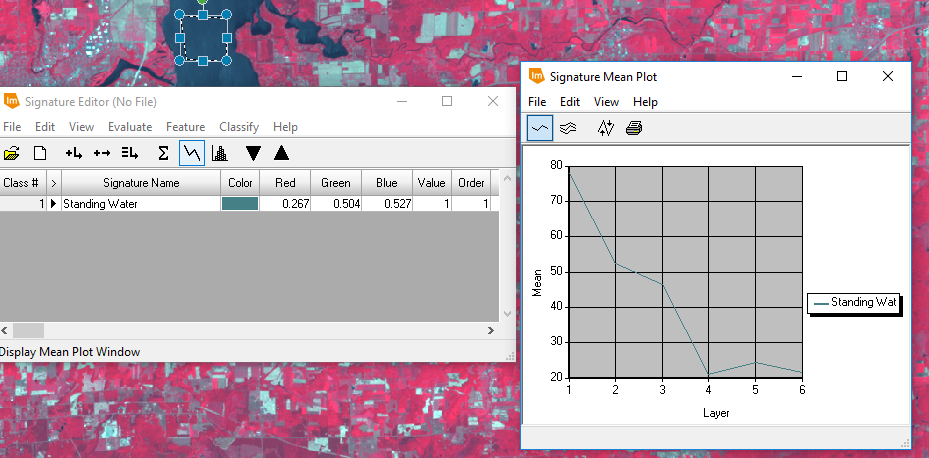 |
| Figure 3: Signature Mean Plot. |
Part 2: Resource Monitoring
For the second part of this lab, a similar multispectral image of the Eau Claire and Chippewa Falls area was used to generate an NDVI and FMI raster. The formula to generate an NDVI is shown in figure 4:
 |
| Figure 4: Formula to generate an NDVI. |
The Raster > Unsupervised > NDVI tool (figure 5) was used to generate indicies for the entire image, rendering more aqueous areas as black and more vegetation cover as white (figure 6).
 |
| Figure 5: Using the NDVI raster tool. |
 |
| Figure 6: Using the Landsat 7 sensor and NDVI index, a new NDVI was generated (see results). |
Next, a similar procedure was followed, only this time, to generate an FMI (figures 7 and 8).
 |
| Figure 7: Formula to generate an FMI. |
 |
| Figure 8: Using the Landsat 7 sensor and ferrous minerals index, an FMI was created (see results). |
 |
| Figure 9: Spectral signatures of all surface features. |
 |
| Figure 10: Dry versus moist soils. |
 |
| Figure 11: NDVI |
 |
| Figure 12: FMI |
Looking at the NDVI and FMI (figures 11 and 12), there are some distinct patterns that are represented by the data. For instance the northeastern half of the image is classified as mostly vegetation in both images. Similarly the cultivated farmlands to the southwest are dominated by ferrous minerals and moisture.
Overall, I found this lab to be an insightful way to learn about differences in spectral reflectances of surface features and a first-hand look at how NDVIs and FMIs are generated using ERDAS; a very powerful software.
Sources
Dr. Cyril Wilson
ERDAS Imagine
ESRI
USGS - Earth Resources Observation and Science Center
No comments:
Post a Comment