Mini Term Project

Introduction

Throughout the duration of this course, a lot of image interpretation functions were covered. The goal for this lab was to use four of those functions on images downloaded from the USGS-GloVis site. The four image functions I chose to do include:
-

Lab 8: Spectral Signature Analysis & Resource Monitoring

Introduction

The goal of this lab was to investigate the reflective properties of surface features and various image index functions using ERDAS Imagine. By using a multispectral image of the Eau Claire and Chippewa Falls area, the spectral properties of the following features were studied:

• Standing water
• Moving water
• Deciduous forest
• Evergreen forest
• Riparian vegetation
• Crops
• Dry Soil (uncultivated land)
• Moist Soil (uncultivated land)
• Rock
• Asphalt highway
• Airport runway
• Concrete bridge

In addition, a normalized difference vegetation index (NDVI) and ferrous minerals index (FMI) were generated using a multispectral image of the same area.

Methods

Part 1: Understanding Spectral Signatures of Surface Features

By first bringing in the multispectral image of Eau Claire to ERDAS Imagine the various surface features aforementioned were identified in the image. This was done by drawing a polygon within the feature area using the Drawing > Polygon tool (figure 1).

Figure 1: Digitizing the area of interest (AOI).

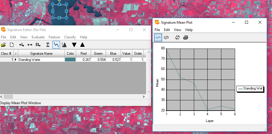
Once the AOI for each feature was drawn, the spectral signatures of each feature were analyzed using the Raster > Supervised > Signature Editor tool (figure 2) and the Signature Mean Plot (SMP) function within the tool (figure 3).

Figure 2: Signature Editor Tool.

Figure 3: Signature Mean Plot. 

In figure three, the x axis of the SMP window represents the different spectral bands reflected by the surface feature and the y axis represents the mean reflectance within that AOI. Each surface feature's SMP could be visualized individually or with multiple graphs in one SMP window (see results).

Part 2: Resource Monitoring

For the second part of this lab, a similar multispectral image of the Eau Claire and Chippewa Falls area was used to generate an NDVI and FMI raster. The formula to generate an NDVI is shown in figure 4:

Figure 4: Formula to generate an NDVI.

The Raster > Unsupervised > NDVI tool (figure 5) was used to generate indicies for the entire image, rendering more aqueous areas as black and more vegetation cover as white (figure 6).

Figure 5: Using the NDVI raster tool.

Figure 6: Using the Landsat 7 sensor and NDVI index, a new NDVI was generated (see results).

Next, a similar procedure was followed, only this time, to generate an FMI (figures 7 and 8).

Figure 7: Formula to generate an FMI.

Figure 8: Using the Landsat 7 sensor and ferrous minerals index, an FMI was created (see results).

Results

Figure 9: Spectral signatures of all surface features.

Figure 10: Dry versus moist soils.

Figure 11: NDVI

Figure 12: FMI

Looking at the spectral signatures of various surface features (figures 9 and 10), the differences in reflectance changed mostly in the blue, red, near-infrared (NIR), and mid-infrared (MIR) spectral bands. As shown in figure 10, dry soil reflects more light than moist soils, specifically in the red band. This is due to the absorption properties of water and could likely also be a reflection of the soil's composition.

Looking at the NDVI and FMI (figures 11 and 12), there are some distinct patterns that are represented by the data. For instance the northeastern half of the image is classified as mostly vegetation in both images. Similarly the cultivated farmlands to the southwest are dominated by ferrous minerals and moisture.

Overall, I found this lab to be an insightful way to learn about differences in spectral reflectances of surface features and a first-hand look at how NDVIs and FMIs are generated using ERDAS; a very powerful software.

Sources


Dr. Cyril Wilson
ERDAS Imagine
ESRI
USGS - Earth Resources Observation and Science Center

Lab 7: Photogrammetry

Introduction

The goal of this lab was to become familiar with tasks and practices associated with photogrammetry of aerial photographs. These tasks consisted of developing scales for and measuring aerial photos, calculating relief displacement of features in aerial photographs, creation of anaglyphs for steroscopy, and geometrically correcting images for orthorectification.

Methods

To complete the first task in this lab, scaling and measruing features of aerial photographs, an aerial image of southwestern Eau Claire was used to determine the distance between two points (figure 1).

Figure 1: Image used for determining ground distance from an aerial photograph.

To do this, a ruler was used to measure the distance between the points on the computer screen, then using the known scale of the photograph to determine the true ground distance. Next, the area of a lake was calculated using the digitizing function on ERDAS.

Figure :

Figure :

Then, a smoke stack that was warped in an aerial image was corrected by calculating the relief displacement of the object (figure 2).

Figure 2: Image used for determining the relief displacement of an object.

The distance from the principal point to the base of the smoke stack as well as the height of the smoke stack was measured and used to calculate the degree of relief displacement.

To achieve the next objective, ERDAS Imagine was used to create anaglyph images of the Eau Claire area. This was done by first using a digital elevation model (DEM) of the area combined with a multispectral image. The Terrain Anaglyph tool was used, which produced 3-D anaglyph image when viewed with red and blue stereoscopic glasses, the terrain became visible in three dimensions. The same process was done with a digital surface model (DSM) instead of the DEM. This version produced a smoother and more accurate 3-dimensional rendering.

Figure 3: Using a multispectral image and DEM to generate a terrain anaglyph image.

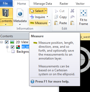
Lastly, two images were orthorectified, which means they were stitched together using ground control points (GCPs) between two images. To achieve this, the first step was to first project each image so that they were in the proper coordinate system.

Figure: Choose projection.

Second, the Sensor Model was defined and each image was added to the image viewer. Each image was then set up for placing ground control points (GCPs) to tie the image down to a reference image.

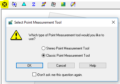Figure : Start Select Point Measurement Tool. 

Figure : Set coordinate system for GCPs using the Reset Horizontal Reference Tool.

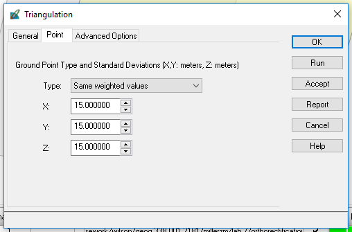Figure : Establish triangulation parameters.

Figure : Add GCPs to the reference and input image using the Create Point Tool.

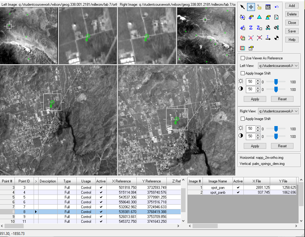Figure : View of overlapping points of the two images after being geometrically corrected.

Then, the GCPs were stitched together using the Automatic Tie Point Generation Properties tool.

Figure : Auto Tie Summary showing results of the image tying.

Results

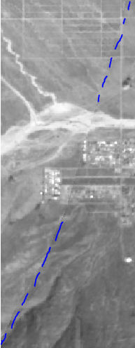Figure : 

The image above represents the two images before orthorectification. Having no spatial reference, the images would lay on top of each other if put into the same viewer and were the same size. After orthorectifying the images, the two images are merged together seamlessly and spatially accurate.

Figure : A zoomed-out view of the orthorectified images.