Lab 6: Geometric Correction

Introduction

The purpose of this lab was to work with and understand geometric correction of rasters. To do this, ERDAS Imagine was used in accordance with a dataset containing multispectral and USGS images and references of Chicago and Sierra Leone.

Methods

In order to achieve the initiatives outlined in the previous section, it was important to understand how geometric correction worked before preforming this action on imagery. In the first part of this lab, a multispectral image of the Chicago area was corrected using a USGS rendering as a reference. Only three ground control points (GCPs) were required since a first-order transformation (figure 1) was used.

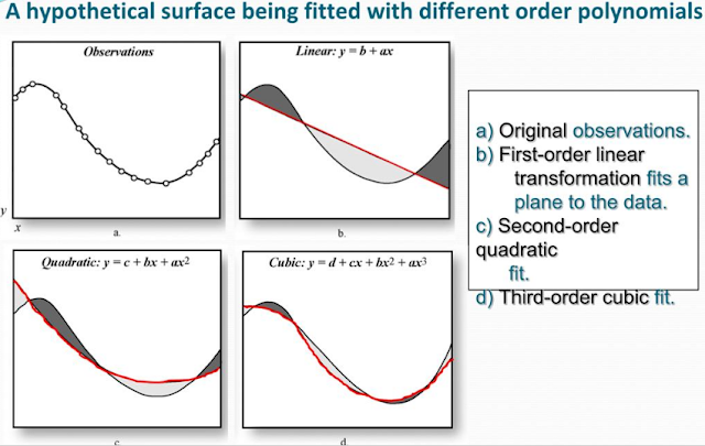Figure 1: Differences of ordered polynomial transformations.

The order of transformation directly relates to the amount of GCPs required for correction, as the averaging becomes more complex and accurate. Using the Multipoint Geometric Correction tool (figure 2) a dialog window opened allowing the geometric process to commence.

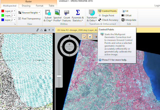Figure 2: Add control points tool.

 When the dialog window opened, a Polynomial Geometric Model was set to ensure 3 GCPs were used in first-order transformation. Then, by clicking the Create GCP button in the dialog window (figure 3), a point was selected in both the multispectral image and the reference map (figure 4).

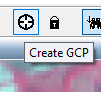Figure 3: Create GCP button in Geometric Correction dialog window.

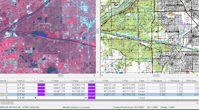Figure 4: GCP #4 shown in both maps.

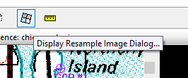
As seen in figure 4, when initially locating the points, they were a bit different between the two images. This was corrected by moving the points around either window until a Control Point Error (bottom right of figure 4) of > 0.5 pixel was achieved. Once the images had accurate GCPs, the geometric correction was performed by creating an output file for the image, setting the resampling method to Nearest Neighbor, and prompting the dialog window to run the calculations based on the GCPs placed in the images (figure 5).

Figure 5: Complete geometric correction. 

In the second part of this lab, geometric correction was performed on a different set of images, this time, two multispectral images of an area in Sierra Leone. One image is quite distorted while the other is geometrically correct, this will serve as a reference for the first image. Following a similar procedure as the previous part, the warped image viewer was selected and the Multipoint Geometric Correction tool was used to add a minimum of nine GCPs to the images. The number of GCPs required for this part was due to the use of a third-ordered transformation.

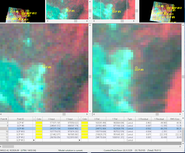Figure 6: Adding GCPs to Sierra Leone images.

When calculating the geometric correction for these images, Bilinear Interpolation was used instead of Nearest Neighbor. Due to the large amount of GCPs used and a desire to preserve as much shape of the reference image as possible, this method was chosen this time around.

Results

Figure 7: Geometrically corrected multispectral image (Part 1).

Figure 8: Original multispectral image (Part 1).

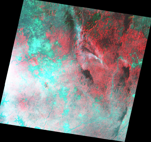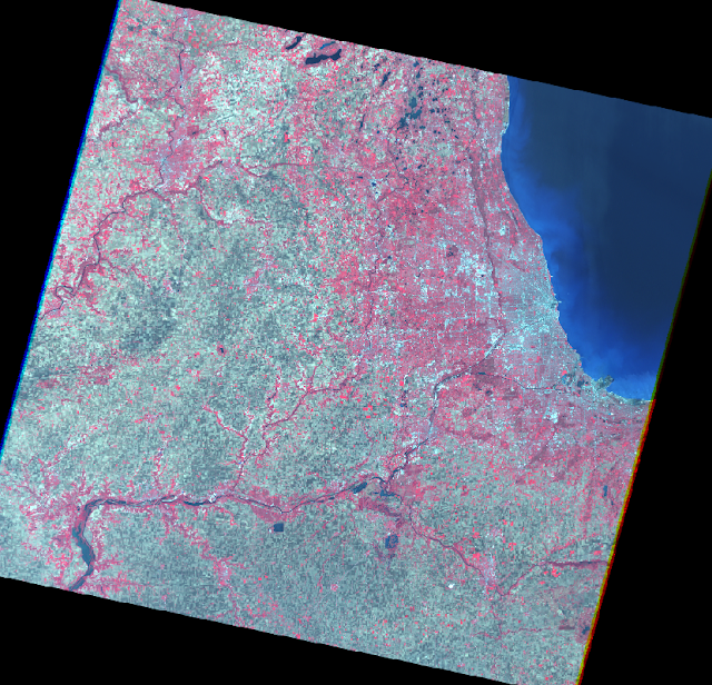
Figure 9: Original multispectral image (Part 2).

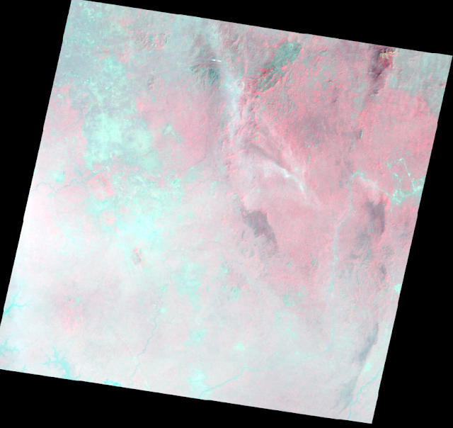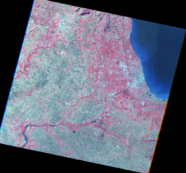
Figure 10: Geometrically corrected multispectral image (Part 2).

Conclusion

Looking at the geometrically corrected images in the results section (figures 8 and 10 respectively), the transformations look vastly different. In the corrected Chicago image (figure 8), the changes are slight. It appears as though the image is almost pushed further away from the viewer, more of Lake Michigan and the southwestern corner of Illinois. The corrected image also appears to pixelate sooner than the original image, so the correction appears to preserve shape while distorting spatial resolution.

As for the second geometrically corrected image (figure 10), similar results to the first part are generated. The image appears further away and the color brilliance/ spatial resolution appears diminished. The size and shapes of features in the corrected image are incredibly close to those of the reference image, however. Perhaps in a professional setting, the two images could be used in accordance with each other to analyze features.

Overall, the geometric correction of multispectral imagery can provide a much more spatially accurate image for remote sensing applications. The process of geometric correction was fairly easy to complete in ERDAS Imagine as the prompts essentially only required input images, GCPs, and a resampling method to correct imagery. The image with more GCPs appeared to be more geometrically accurate than the first corrected image which only used 4 GCPs.

Lab 5: LiDAR Remote Sensing

Introduction

The purpose of this lab was to become familiar with using LiDAR (light detection and radar) data for remote sensing applications. Using ERDAS Imagine and ArcMap to visualize the point cloud information.

Methods

Using a folder containing 40 lidar data files, the quarter section tile data was brought into ERDAS Imagine to visualize them as point cloud data. The files were exported to a project folder as .las (point cloud tiles) files.

Figure 1: Add .las files to ERDAS Imagine.

Once the files LAS as Point Cloud files were saved, an LAS Dataset was created in ArcMap. This was done by adding the point cloud files to the LAS dataset prompt and calculating statistics about the data comprising the files.

Figure 2: Create new LAS dataset in ArcMap.

Figure 3: Add files to LAS dataset in ArcMap.

This calculation returned information regarding the highest and lowest Z-values (elevation) of the study area's returns, and classified the return values. The dataset was projected into a horizontal and vertical coordinate system since the point cloud data contained X,Y, and Z coordinates.

Figure 4: Choose horizontal coordinate system for LAS dataset.

Figure 5: Choose vertical coordinate system for LAS dataset.

The dataset was then used in ArcMap to visualize the point cloud in various ways. By navigating to the symbology tab within the dataset layer properties, the number of classes, which returns, colors, and other parameters were configured to visualize the dataset for different applications.

Figure 6: Visualizing the lidar point cloud in ArcMap.

Using the LAS Toolbar was helpful in interpreting various components of the dataset. The profile tool was especially helpful in determining false return points within the point cloud.

Figure 7: Using the profile tool in ArcMap.

Next, a Digital Surface Model, Digital Terrain Model, and corresponding Hillshades were created using the dataset. To achieve this, the LAS Dataset to Raster tool was used, adjusting different components within the prompt to display surface or terrain.

Figure 8: Using LAS Dataset to Raster tool in ArcMap to create a Digital Terrain Model (DTM).

Figure 9: Using LAS Dataset to Raster tool in ArcMap to create a Digital Surface Model (DSM) using the first return of point cloud. 

Lastly, an Intensity Image was created using the intensity values within the dataset instead of elevation values. The image was then brought into ERDAS Imagine for better visualization.

Results

Figure 10: Digital Surface Model result.

Figure 11: Digital Terrain Model result.

Figure 12: Intensity image result.

Discussion

I found the lidar visualization skills learned in this assignment were interesting and beneficial. Having never worked with a lidar dataset before this assignment, I now feel more confident in my ability to work with these types of datasets. Of course, this lab covered basic functionalities and visualization techniques for lidar datasets, however, lidar now seems more exciting and useful of a technology for visual interpretation, land use/land cover, and other remote sensing applications than satellite imagery. There are benefits to using either technology and, in some cases, could be used in accordance with one another. LiDAR datasets are indeed more versatile than satellite imagery, due to their Z coordinate values, return layers, and profile viewing capabilites alone- you just can't get that level of 3-dimensional information with satellite imagery.